Rossman Store Sales Prediction
When you want to practice your Data Science skills, there’s nothing better than getting your hand dirty with a Kaggle-style tabular data challenge.
In this post I give an overview of a project I did while at the Data Science Retreat Berlin together with my team mates Maryam Faramarzi and Naveen Korra.
Summary
This post contains a brief description of the analysis done and the final model.
You can find the full code for the project on GitHub. There you can also find notebooks with detailed explanations of the modeling.
Task
The goal of this project was to predict the sales number of Rossman stores over time. The data was adapted from the Kaggle Rossman challenge. It includes the daily sales number of Rossman stores from January 2014 to July 2015.
In addition, information on the individual stores is provided, such as the type of store, the assortment of items sold, etc.
Result
We performed data exploration, data cleaning and feature engineering of the original Rossman store data.
We then trained several models, including Linear Regression, Random Forest Regressors and Gradient Boosted Trees, and performed hyperparameter optimization.
To evaluate the models we used the root mean square percentage error ($\mathrm{RMSPE}$), which gives the average percentual error between the actual sales $y_i$ and the predicted sales $\hat{y}_i$.
$$ \mathrm{RMSPE}=\sqrt{ \frac{1}{n} \sum_{i=1}^n \left(\frac{y_i-\hat{y}_i}{y_i} \right)^2 } $$
| Model | $\mathrm{RMSPE}$ |
|---|---|
| Naive model (mean) | 62.03 |
| Linear Regression | 22.81 |
| Random Forest | 17.07 |
| Gradient Boosted Trees | 12.38 |
The best performing model was a Gradient Boosted Tree implemented with the LightGBM library. On the holdout dataset of the competition, the GBT achieved an RMSPE of 16.17%.
Here’s a comparison of prediction vs. actual sales per day:
Detailed Explanation
Here is a walk-through of the project. The following table of contents gives an overview of what we did, and you can use it to jump to specific parts.
Table of Contents
Data Processing
import numpy as np
import pandas as pd
import matplotlib
import matplotlib.pyplot as plt
matplotlib.rcParams['figure.dpi']=150
import plotly.express as px
import plotly.graph_objects as go
from datetime import datetime
# Load scripts from parent path
import sys, os
sys.path.insert(0, os.path.abspath('..'))
# Ignore some future warnings triggered when training
import warnings
warnings.filterwarnings(action="ignore", category=FutureWarning)
Load raw sales data
First we load the table that contains the raw daily sales by Rossmann store.
The target column is:
Sales: The total sum of sales for this store and date
The features columns are:
Date: The date of the sales recordStore: An ID of the storeDayOfWeek: The day of the week, given as an integer, ranging from Monday (0) to Sunday (6).Customers: The number of customers for this store and date. We will drop this, as this information is not available for the future.Open: Whether the store was open on this date: 0 = closed, 1 = openPromo: Whether the store ran a promotion on this date.StateHoliday: Whether this date was a state holiday.SchoolHoliday: Whether this date was a school holiday.
The training data includes data for one and a half years, from 2013-01-01 until 2014-07-31.
The holdout (test) period is the following 6 months, from 2014-08-01 to 2015-07-31.
train_raw = pd.read_csv("../data/train.csv", parse_dates=[0])
train_raw.head()
| Date | Store | DayOfWeek | Sales | Customers | Open | Promo | StateHoliday | SchoolHoliday | |
|---|---|---|---|---|---|---|---|---|---|
| 0 | 2013-01-01 | 1115.0 | 2.0 | 0.0 | 0.0 | 0.0 | 0.0 | a | 1.0 |
| 1 | 2013-01-01 | 379.0 | 2.0 | 0.0 | 0.0 | 0.0 | 0.0 | a | 1.0 |
| 2 | 2013-01-01 | 378.0 | 2.0 | 0.0 | 0.0 | 0.0 | 0.0 | a | 1.0 |
| 3 | 2013-01-01 | 377.0 | 2.0 | 0.0 | 0.0 | 0.0 | 0.0 | a | 1.0 |
| 4 | 2013-01-01 | 376.0 | 2.0 | 0.0 | 0.0 | 0.0 | 0.0 | a | 1.0 |
Let’s have a look at the correlation of the features. There is a relatively high correlation between sales and promotions. But most other numerical features are not very correlated. Therefore, we keep all of them for now.
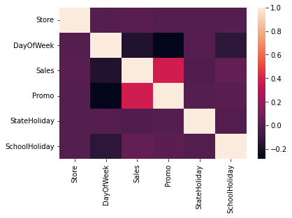
Figure: The correlation matrix of the raw features.
Plot sales
Let’s just look at the daily sales numbers over time.
sales = train_raw.groupby(by='Date').agg({'Sales': 'sum'}).reset_index()
fig = go.Figure()
fig.add_trace(go.Scatter(x=sales['Date'], y=sales['Sales'],
mode='lines+markers',
name='actual'))
fig.update_layout(title='Sales over Time',
xaxis_title='Date',
yaxis_title='Total Sales')
fig.show()
As we see, there is a strong weekly seasonality. Sales on Sunday and Saturday are very small.
Also, there does not seem to be a strong trend over time, so we don’t have to account for this for now.
We’ll now go over to some feature engineering. For more details on the data, have a look at the Data Exploration notebook in the Github repository.
Add features: months, weeks
The Date-column in itself is not informative, as our prediction should
extrapolate in the future. However, features of the date can be extracted.
To capture seasonal trends in sales, we added the features:
month: The month of the year.week: The week of the year.
def add_week_month_info(train):
"""
Add week and month information as another column to the features.
"""
train.loc[:,'week'] = train.loc[:,'Date'].dt.isocalendar().week.astype(int)
train.loc[:,'month'] = train.loc[:,'Date'].dt.month
return train
train = add_week_month_info(train_raw)
Add features: Beggining and end of month signifiers
After our first round of modeling, we analyzed the errors/residuals of our model over time and found something interesting: The model was often wrong towards the beginning and end of months (see chapter Prediction and Error Analysis).
This indicates that there is a periodical influence that affects sales at the beginning and end of months (for example if people receive their paycheck with some regularity).
To enable our model to learn these patterns, we added features that signify the beginning and end of months:
beginning_of_month: Indicates whether the date is towards the beginning of the month, ranging from 0 (no) to 1 (yes).end_of_month: Indicates whether the date is towards the end of the month, ranging from 0 (no) to 1 (yes).
def add_beginning_end_month(train):
"""
Add features that represent the beginning and end of months.
"""
def get_feature_end_month(day_of_month):
return (day_of_month/31)**4
def get_feature_beginning_month(day_of_month):
return ((31-day_of_month)/31)**4
# get_feature_end_month(33)
train.loc[:, 'end_of_month'] = train.loc[:, 'Date'].dt.day.apply(get_feature_end_month)
train.loc[:, 'beginning_of_month'] = train.loc[:, 'Date'].dt.day.apply(get_feature_beginning_month)
return train
train = add_beginning_end_month(train)
Visualization of beginning/end of month features
month_features = train.groupby(by='Date').agg({'end_of_month': 'first', 'beginning_of_month': 'first'}).reset_index()
fig = go.Figure()
fig.add_trace(go.Scatter(x=month_features['Date'], y=month_features['end_of_month'],
mode='lines',
name='end_of_month'))
fig.add_trace(go.Scatter(x=month_features['Date'], y=month_features['beginning_of_month'],
mode='lines',
name='beginning_of_month'))
fig.update_layout(title='End/Beginning of month features over time',
xaxis_title='Date',
yaxis_title='value',
xaxis_range=[datetime(2013, 3, 1),
datetime(2013, 7, 1)])
fig.show('png')
Clean data
Before starting with modeling, we do some small data cleaning steps:
- Drop the
Customerscolumn, as this info will not be available in the future. - Remove rows with sales that are null or 0.
- Drop the
Opencolumn - stores that have non-zero sales are open. - Remove observations with null values in any feature.
- etc.
def clean_data(train_raw, drop_null=True, drop_date=True):
""" Some common basic data processing.
This function
- Encodes the state holidays
- Drops unneeded columns (Customers, Open, Date)
- Removes all rows where 'Sales' were 0
- Removes all rows with nan values
"""
train = train_raw.copy()
train.loc[:, 'StateHoliday'] = train.loc[:, 'StateHoliday'].replace(to_replace='0', value='d')
train.loc[:, 'StateHoliday'].replace({'a':1, 'b':2, 'c':3, 'd':4}, inplace = True)
# Drop customers, open and Date
train = train.drop(["Customers", "Open"], axis=1)
if drop_date:
train = train.drop("Date", axis=1)
# Drop all where sales are nan or 0
if 'Sales' in train.columns:
train = train.dropna(axis=0, how='any', subset=['Sales'])
train = train.loc[train.loc[:, 'Sales']!=0, :]
# Drop all null value
if drop_null:
train = train.dropna(axis=0, how='any')
return train
train = clean_data(train)
Add features: Store info
Some additional information on the stores was made available in the
file data/store.csv.
We combined this with the sales information and calculated some additional features which we add to the sales information (for details see the GitHub repository):
Store: The ID of the store, for mapping to the sales data.StoreType: The type of store, differing between four models, a, b, c, d.Assortment: The type of goods that the store is carrying, a = basic, b = extra, c = extended.CompetitionDistance: The distance to the nearest competing store, in meters.month: The month for which average sales and customers were calculated.Store_Sales_mean: The mean sales for this store and month.Store_Customers_mean: The mean customers for this store and month.
def add_store_info(train):
""" Add the store info to sales data.
Merges the store info on the train table and returns the combined table
"""
# Load store info
store_info = pd.read_csv("../data/store_info.csv")
# Merge store info onto train data
train = pd.merge(left=train, right=store_info, how='left', on=['Store', 'month'])
return train
train = add_store_info(train)
train.loc[:, ['StoreType', 'Assortment',
'CompetitionDistance', 'Store_Sales_mean',
'Store_Customers_mean']].head()
| StoreType | Assortment | CompetitionDistance | Store_Sales_mean | Store_Customers_mean | |
|---|---|---|---|---|---|
| 0 | b | b | 900.0 | 4139.474576 | 1153.783333 |
| 1 | b | a | 90.0 | 12845.896552 | 2384.271186 |
| 2 | b | b | 590.0 | 3725.649123 | 888.627119 |
| 3 | b | a | 1260.0 | 7079.150000 | 1010.583333 |
| 4 | a | c | 18160.0 | 2260.783333 | 333.610169 |
Model Training
Prepare train/test data
Now let’s get started with modeling! First, we prepare the final dataset the training.
The target label is Sales.
The features are all the other columns in the dataset.
# Split label and features
X = train.copy(deep=True).drop(columns=["Sales"])
y = train.loc[:, "Sales"]
# Make train test split
from sklearn.model_selection import train_test_split
X_train, X_test, y_train, y_test = train_test_split(X, y, test_size=0.2)
X.head()
| Store | DayOfWeek | Promo | StateHoliday | SchoolHoliday | week | month | end_of_month | beginning_of_month | StoreType | Assortment | CompetitionDistance | Store_Sales_mean | Store_Customers_mean | |
|---|---|---|---|---|---|---|---|---|---|---|---|---|---|---|
| 0 | 353.0 | 2.0 | 0.0 | 1.0 | 1.0 | 1 | 1 | 0.000001 | 0.877078 | b | b | 900.0 | 4139.474576 | 1153.783333 |
| 1 | 335.0 | 2.0 | 0.0 | 1.0 | 1.0 | 1 | 1 | 0.000001 | 0.877078 | b | a | 90.0 | 12845.896552 | 2384.271186 |
| 2 | 512.0 | 2.0 | 0.0 | 1.0 | 1.0 | 1 | 1 | 0.000001 | 0.877078 | b | b | 590.0 | 3725.649123 | 888.627119 |
| 3 | 494.0 | 2.0 | 0.0 | 1.0 | 1.0 | 1 | 1 | 0.000001 | 0.877078 | b | a | 1260.0 | 7079.150000 | 1010.583333 |
| 4 | 530.0 | 2.0 | 0.0 | 1.0 | 1.0 | 1 | 1 | 0.000001 | 0.877078 | a | c | 18160.0 | 2260.783333 | 333.610169 |
Feature Encoding
We originally used one-hot encoding for certain features such as Assortment type, State holiday, Store type. However, we found that the model performance increased when choosing target encoding for all categorical features.
import category_encoders as ce
target_encode = ce.TargetEncoder()
Feature Scaling
In addition, applied standard scaling to all features. This is mostly important for the linear regression model.
from sklearn.preprocessing import StandardScaler
scaler = StandardScaler()
Model Selection
We applied various different models, including
- Naive Mean Estimator (to create a baseline)
- Linear Regression
- Random Forest Regressor
- Gradient Boosted Trees
We found that the best performing model was a Gradient Boosted Tree (GBT),
which we trained using the LightGBM library.
Here, we only show the training of this final model.
You can find details on the training of the other models in the notebooks:
We also performed a hyperparameter optimization of the GBT model. We only show the final best parameters here, for details on the optimization see the notebook notebooks/3_advanced_models.
from lightgbm import LGBMRegressor
# Create GBT model with best parameters (from hyperparameter optimization)
model = LGBMRegressor(
n_estimators=500,
max_depth=25,
num_leaves=80
)
Training the pipeline
We created a pipeline consisting of different processing steps: encoding, scaling and modeling
from sklearn.model_selection import GridSearchCV
from sklearn.pipeline import Pipeline
pipe = Pipeline(steps=[
('target_encode', target_encode),
('scaler',scaler),
('model',model)])
pipe.fit(X_train, y_train)
Pipeline(steps=[('target_encode',
TargetEncoder(cols=['StoreType', 'Assortment'])),
('scaler', StandardScaler()),
('model',
LGBMRegressor(max_depth=25, n_estimators=500, num_leaves=80))])
Model Performance
Finally, we evaluated the error using on the test data set.
from scripts.processing import metric
y_pred_train = pipe.predict(X_train)
y_pred = pipe.predict(X_test)
rmspe = metric(y_test.values, y_pred)
print(f"RMSPE metric on test set: {rmspe:.2f}")
RMSPE metric on test set: 12.38
This root mean square percentage error means that the average percentual error between the actual sales $y_i$ and the predicted sales $\hat{y}_i$ is 12.38%, which is quite good for our inital approach.
Final Training
Finally, we used the best model and trained it once again on the total data to create the final model, and save it for later use
pipe.fit(X, y)
from scripts.pipeline import save_pipeline
save_pipeline(pipeline=pipe, name='LGBM_hyperparam_optim_3')
pipe
Pipeline(steps=[('target_encode',
TargetEncoder(cols=['StoreType', 'Assortment'])),
('scaler', StandardScaler()),
('model',
LGBMRegressor(max_depth=25, n_estimators=500, num_leaves=80))])
Model Evaluation
Prediction and Error analysis
Let’s evaluate the model a bit more. First, we are interested in which time periods the model predicts well, and where it has troubles.
To this end, we calculate the daily model predictions and the error to the actual sales numbers.
def metric_not_summed(preds, actuals):
""" The RMSPE metric per observation """
preds = preds.reshape(-1)
actuals = actuals.reshape(-1)
assert preds.shape == actuals.shape
return 100 * (actuals - preds) / actuals
# Get predictions of the model over the full range of data.
y_pred = pipe.predict(X)
# Load the dates from the data
train_raw = scr.load_train_data()
dates = pd.DataFrame(scr.process_data(train_raw, drop_null=True, drop_date=False).loc[:, 'Date'])
# Merge predicted and actual values
result = dates.copy()
result = result.reset_index() #added step to solve the problem with keys and nan values in y_actual
result.loc[:, 'pred'] = y_pred
result.loc[:, 'actual'] = y
# Sum up result by date
result = result.groupby(by='Date').sum().reset_index()
# Calculate the error
result.loc[:, 'error'] = metric_not_summed(result.loc[:, 'pred'].values, result.loc[:, 'actual'].values)
result.loc[:, 'error_abs'] = np.abs(result.loc[:, 'error'])
result.head()
| Date | index | pred | actual | error | error_abs | |
|---|---|---|---|---|---|---|
| 0 | 2013-01-01 | 7453 | 1.247358e+05 | 87980.0 | -41.777470 | 41.777470 |
| 1 | 2013-01-02 | 1538235 | 5.706822e+06 | 5707185.0 | 0.006356 | 0.006356 |
| 2 | 2013-01-03 | 2521226 | 5.233531e+06 | 5177894.0 | -1.074515 | 1.074515 |
| 3 | 2013-01-04 | 3657192 | 5.629987e+06 | 5627268.0 | -0.048311 | 0.048311 |
| 4 | 2013-01-05 | 4645127 | 5.017485e+06 | 4960593.0 | -1.146888 | 1.146888 |
For a first look, we plot the daily sales numbers predicted by our model with the actual daily sales.
import plotly.express as px
import plotly.graph_objects as go
fig = go.Figure()
fig.add_trace(go.Scatter(x=result['Date'], y=result['actual'],
mode='lines+markers',
name='actual'))
fig.add_trace(go.Scatter(x=result['Date'], y=result['pred'],
mode='lines',
name='predicted'))
# Edit the layout
fig.update_layout(title='Sales over Time - Prediction of Final Model vs. Actual',
xaxis_title='Date',
yaxis_title='Total Sales')
fig.show('png')
We see that predicted and actual sales are very close to each other when aggregated daily. In fact, the plot does not tell us a lot about what our model gets wrong, which is why we look at the error in more detail in the next step.
However, we can draw a few conclusions from the above plot:
- There are no clearly visible time periods where the model performs worse. There is also no visible trend, so that is good.
- We know that our model is on average 12.28% off compared to actual sales, but from daily sales numbers it doesn’t seem that way. Thus, the deviation must be stronger on a store-by-store level. It might be good to look closer at which types of stores the model gets wrong, and why.
Plot errors/residuals
During training, we analyzed the errors/residuals to see which dates the model got wrong, and adpated our features accordingly.
For example, we saw that the model had difficulties predicting sales at the beginning and the end of months, which is why we introduced the beggining/end of month features above.
fig = go.Figure()
fig.add_trace(go.Scatter(x=result['Date'], y=result['error'],
mode='markers',
name='actual'))
fig.update_layout(title='Error over Time',
xaxis_title='Date',
yaxis_title='Error')
fig.show('png')
At the moment there are still some date ranges with larger errors, for example around Christmas and New Years. It is likely that the current features don’t accurately capture holidays, because they only mark the dates of the holiday, but not the adjacent dates. This offers ample space to further improve the model performance.
Feature importance
We also analyzed the importance of features in the final model.
model = pipe['model']
importances = pd.DataFrame({'feature': pipe[1].get_feature_names_out(), 'importance': model.feature_importances_})
importances = importances.sort_values(by='importance', ascending=True)
plt.barh(y=importances['feature'], width=importances['importance'])
plt.xlabel("feature_importance")
plt.show()
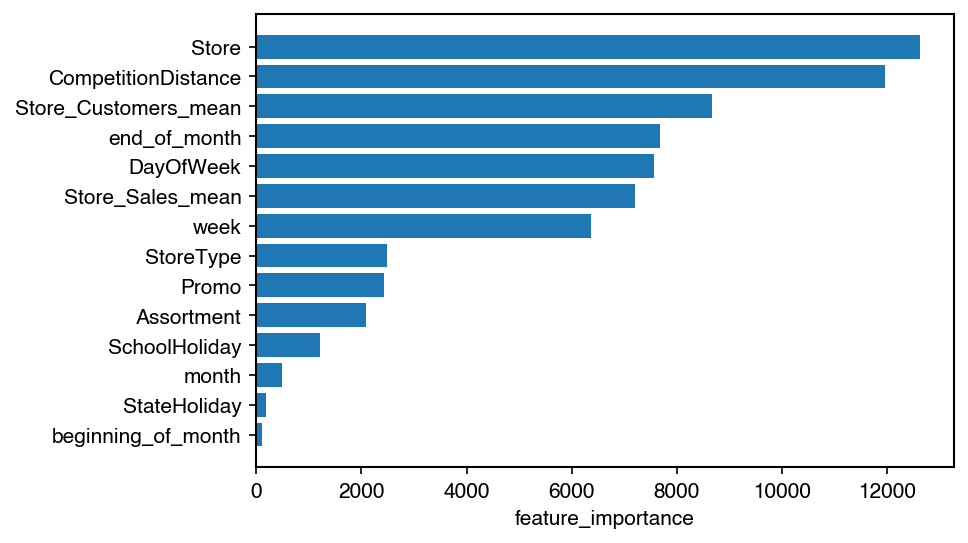
Some interesting insights:
- It appears that the specific store is a very important predictor, as it
features in many variables (
Store,CompetitionDistance, etc.). Some further analysis of the stores should be helpful here. - The
end_of_monthfeature ranks quite high, which indicates that it actually improved model performace.beginning_of_monthis less important. - The holiday-encoding variables
SchoolHolidayandStateHolidayare very low in importance. However, from looking at the sales we know that holidays are important, for example in the elevated sales in December. It might be that these existing variables do not capture these features well. One problem might be that they only indicate the date of the holiday itself, while sales are distorted in a wider period around the holiday. Adding more time-dependent features might help here.
Summary
Overall, the final Gradient Boosted Trees Regression model showed a good performance on both test and holdout set and proved a great starting model.
There found several directions for future work which could help further improve the prediction, mainly:
- analyzing the error on a store-by-store basis, to find which stores the model has problems with
- incorporating holidays better by engineering features that represent these time frames
Thank you for reading! If you want to delve deeper, you can find the full code for the project on GitHub, including additional explanatory notebooks, the data and the full code for reproducing the modeling.